I’m not a very good cook.
I’ve learnt to produce a handful of family meals, which revolve around deterministic cook times and require limited judgement. Pasta. A roast. A stir-fry if I’m feeling ambitious. Basically, I can follow a procedure, but I can’t create anything wonderful.
Something I did notice though was that I can generally produce a uniform pile of chopped herbs or spinach without really thinking about it. I do this by taking a knife to the ingredients and hunting down the largest chunk, making a chop over the pile, then repeating until it looks right.
What I didn’t clock was that I had actually developed a strategy. An algorithm, even.
This thought lodged in my brain while I was halfway through a bag of baby spinach. Why does that approach work? And could I model it?
This page documents what I explored and what I learnt along the way.
Contents
- The question
- Building the simulator
- The mathematics
- Building the compute grid
- 40,320 tasks
- Symbolic regression
- What the data found
- Calculators
- Known limitations
- Glossary
- Further reading
The question
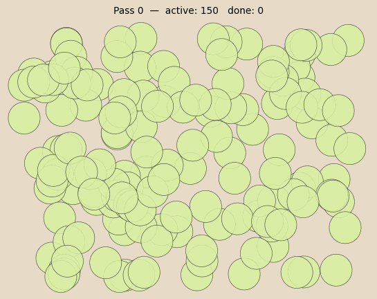
When you chop a pile of herbs, you are probably solving an optimisation problem without realising it. The knife comes down on a scattered pile, you chop a bunch in all directions, scrape everything back together, and repeat. Chop, chop. Chop…
The question is: how many passes does it take?
The answer depends on several things: how many leaves you started with, how fine you need to chop them, how many cuts you make per pass, the size of each leaf, and the size of your chopping board. These are all measurable. The relationship between them should, in principle, have a formula.
Building the simulator
Before trying to derive anything analytically, I built a simulator to generate ground-truth data for any parameter combination. The simulator models the chopping board as a 2D plane, represents leaves as polygons, and applies straight-line cuts one at a time.
Polygon representation
Each leaf is approximated as a 48-sided polygon - this was a tad easier than working with true circle geometry and close enough to work for this problem. Why 48? It is divisible by 4, 6, 8, and 12, which means cuts at common angles (horizontal, vertical, 45°) produce geometrically clean children. The number of sides does not need to be exact; it just needs to be high enough that the approximation does not introduce meaningful area error.
Each polygon is stored as an ordered list of 2D vertices in counter-clockwise winding order. The area is computed once using the shoelace formula and cached:
Originally I had not cached these values, but after a few runs it became clear that for a simulation running thousands of passes with hundreds of fragments, recomputing every piece’s area on every cut was adding up. Since rotation and translation do not change area, the cached value can be carried through repositioning operations and only discarded when a cut produces new child shapes.
Cutting polygons
Each knife pass applies straight-line cuts across the board.
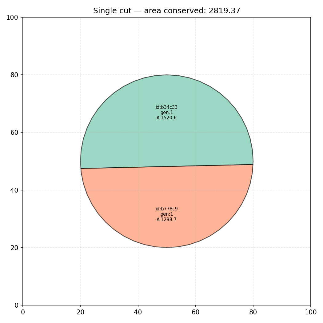
The fundamental operation is splitting a polygon with a straight line. Think of it this way: once you draw a line across the board, every corner (vertex) of a polygon is either to the left of the line or to the right of it. The corners to the left form the left-hand child fragment; the corners to the right form the right-hand child. Where the cut line crosses one of the polygon’s edges, a new corner is created at that exact crossing point and added to both children, so each child is a complete, closed shape.
The maths for deciding which side a corner sits on is straightforward. A straight line can be described by its angle and its distance from the centre of the board. For each corner at position , we compute a single number:
Where is the angle of the cut line and is how far the line is from the origin. This number is positive when the corner is on one side of the line and negative when it is on the other. Corners with go to one child; corners with go to the other.
When consecutive corners sit on opposite sides of the cut (one positive, one negative), the edge between them must cross the cut line somewhere. The crossing point is found by linear interpolation along that edge and added as a new corner to both children. This ensures neither child has a gap where the knife went through.
This is a simplified version of the Sutherland-Hodgman algorithm, a classical computational geometry technique for clipping polygons against a line.
If the cut line misses a polygon entirely, every corner has the same sign and no split occurs. The polygon is returned unchanged.
In the primary simulation mode, each cut is guaranteed to intersect the current largest piece. The angle is random, but the position of the cut line is chosen to fall somewhere within the extent of the largest fragment. This implements the “hunt the largest piece” strategy.
The pile
After each pass, fragments smaller than times their original leaf area are retired to a done bin. The remaining pieces are collapsed into a central heap. The pile geometry is physically motivated: a cook scrapes everything back to the centre before the next pass. Pieces are repositioned within a circle of radius proportional to the square root of total remaining area, with random rotation and placement.
There was a part of me that wanted to track generational fragment lineages and never retire anything to a bin, but I had already taken this idea quite far enough.
The pile radius turned out to be the most important modelling decision in the whole project. More on that in the next section.
Running headless
After running a few local simulations to check the behaviour, I needed to run thousands of them across a range of parameters without any of the visual output. Adding a render=False flag strips out all matplotlib and animation work; a simulation that takes several seconds with visuals runs in under 20ms without them. This is the version the compute grid runs.
# core simulation loop
for pass_num in range(1, n_passes + 1):
    for _ in range(cuts_per_pass):
        active = board_cut(active, board_w, board_h, mode="target_largest")
    active, done = retire_done(active, done, threshold)
    active = collapse_to_pile(active, board_w, board_h, ...)
    if not active:
        finish_pass = pass_num
        break
The output is finish_pass: the pass number on which the last fragment was retired. This is the number the formula needs to predict.
The mathematics
Two phases
Chopping leaves until each fragment is no more than times its original size happens in two distinct phases:
-
Warm-up. Every original leaf must be cut at least once before any fragment can reach the target size. This phase ends when all leaves have been touched by the knife at least once.
-
Refinement. Once every leaf has been hit, the process shifts to reducing each fragment down to the target size. This takes a predictable number of additional passes per fragment.
The total pass count is roughly the sum of these two phases, scaled by the geometry of the pile.
Phase 1: the coupon collector
The warm-up phase follows the structure of a well-known probability puzzle: if you have different types of playing cards and you draw one at random each time (replacing it each time), how many draws does it take before you have seen every type at least once?
At the start, every card you draw is a new one so progress is fast. But as your collection grows, more and more draws land on cards you have already seen. When you are missing just one type out of , each draw has only a 1-in- chance of being the card you need. You can end up drawing the same familiar cards many times before that last one finally appears. The total expected wait turns out to grow as - the natural logarithm of .
To make that concrete: , , . Doubling the number of leaves does not double the warm-up cost; it only adds passes. This slow growth is why the formula is manageable at all. Multiplying the leave count by 1000 adds fewer than five passes to the warm-up.
In the chopping problem, each pass plays the role of a card draw. The knife sweeps across the pile and hits each piece with a probability roughly proportional to its size relative to the pile. Larger pieces are more likely to be caught; smaller fragments can escape a given pass entirely. The target-largest strategy guarantees that the biggest remaining piece is always cut, but the other pieces it happens to catch on that same sweep are essentially random. On average, it takes approximately passes before every original leaf has been cut at least once.
This term is the dominant contribution to the formula for any reasonably large . It was also one of the first things confirmed when I later ran symbolic regression on the simulation data. Without any structural hints, the very first meaningful expression the algorithm found was which is just the logarithm multiplied by a constant, nothing else. The coupon-collector structure was already visible in the data before I had told it to look there.
Phase 2: the binary tree recursion
Once every leaf has been touched, we need each fragment to shrink to below times its original area.
Consider a single leaf of area . A random straight-line cut through a circle divides it into two pieces. Integrating over all possible cut positions, the expected area of the larger piece is and the smaller piece . This ratio is the key number.
For the target-largest strategy, each cut goes to the current biggest piece. The number of cuts needed to reduce a single leaf from area to below the threshold is approximately:
Reading that out loud: how many times do you need to multiply by before the result drops below ? The ceiling symbol means we round up to the nearest whole number, because you cannot make a fraction of a cut. The denominator is the expected reduction per cut.
Not all of those cuts happen on the same pass, though. On any given pass, only some fragments are large enough to be worth targeting. The number of additional passes needed after the warm-up, accounting for how many fragments are being actively reduced at once, is:
The in the denominator is a correction for fine thresholds. When is small (very fine chop), a larger proportion of fragments are simultaneously close to the threshold and being reduced in parallel, which speeds up the refinement phase. When is large (coarse chop), fewer fragments are near the threshold at any one time, so the denominator is just 1.
The pile geometry
Both phases happen in the context of a pile with a physical radius. A larger pile means the knife covers a smaller fraction of it per cut, so more passes are needed to work through everything. The formula’s dependence on pile radius is direct and linear: double the pile radius, double the passes.
The pile radius is whichever is smaller: the size the pile would naturally form, or the size the board allows.
Where is leaf radius, is the pile packing density, and and are board dimensions. The subtracted 1 cm provides a small margin from the edge.
is what the pile radius would be on an infinitely large board: it grows with the square root of (more pieces, bigger pile) and with leaf size. is the physical limit imposed by the board edge.
I initially used everywhere, reasoning that the pile would always fill the available space. For small numbers of large leaves on a big board, the pile never actually reaches the board edge, instead it sits in the centre, much smaller than the board constraint would suggest. Using the board radius in that case is equivalent to telling the formula the pile is several times larger than it actually is. The knife is predicted to make far more passes than needed, because the model thinks it is working through a much bigger heap.
This single wrong assumption I made where I was treating every simulation as board-constrained regardless of how many leaves were actually in it produced an of 0.53 when I tested the formula against 4,032 parameter combinations. Nearly half of all variance was unexplained. Switching to lifted to 0.84. A single line change in the feature engineering step (of PySR) recovered 31 percentage points of explained variance. It is a good example of a modelling error that looks minor on paper but dominates empirical performance.
The transition point is where - the leaf count above which the board edge becomes the constraint:
For a standard 40x30 cm board with 1.75 cm radius leaves, . Any simulation with more than 35 leaves is board-constrained; fewer than 35 and the pile is free. The board constraint checker later in this page computes this for any setup.
The complete formula
Combining both phases with the pile geometry:
Where:
- is the predicted number of passes
- is the effective pile radius
- is the warm-up term (coupon collector)
- is the refinement term
- is the number of cuts per chain
- is cuts per pass
- is leaf radius in cm
The formula says: passes are proportional to pile radius, inversely proportional to cuts per pass, inversely proportional to leaf size, and scale with a combined -and-threshold term.
Building the compute grid
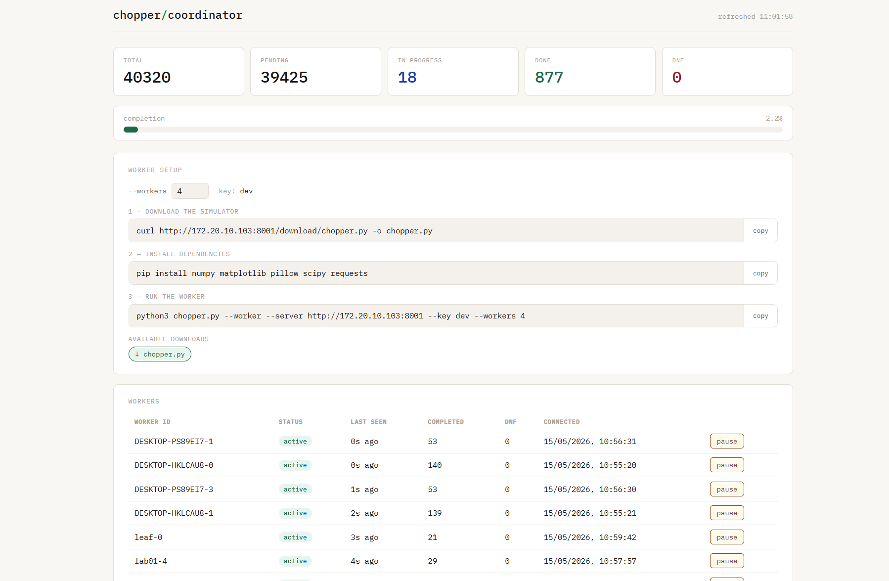
With a formula derived, the next step was validating it across a large parameter space. A single simulation runs in 0.02 to 35 seconds depending on parameters. Running 40,000 of them needs a grid.
Architecture
The grid splits into a coordinator and workers. The coordinator is a FastAPI application running on a Windows machine, backed by SQLite. Workers are a single Python script that can run on any machine with network access to the coordinator.
coordinator  (Windows, FastAPI + SQLite)
    |
    |----HTTP----+----HTTP----+----HTTP----+
    |            |            |            |
 laptop       server       desktop     desktop
 (WSL2)      (Linux)      (Windows)   (Windows)
Each worker spawns one process per CPU core. Processes claim tasks from the coordinator, run them locally, and submit results. The coordinator tracks progress, handles timeouts, and serves a live dashboard.
The concurrency challenge: claiming tasks
The first non-trivial problem was claiming tasks without race conditions. If two workers simultaneously ask for the next pending task, they could both receive the same task and both run it, wasting compute and producing duplicates.
The solution is an atomic claim using SQLite’s BEGIN IMMEDIATE transaction, which acquires an exclusive write lock at the start of the transaction rather than at the first write:
conn.execute("BEGIN IMMEDIATE")
task = conn.execute(
    "SELECT * FROM tasks WHERE status='pending' ORDER BY created_at LIMIT 1"
).fetchone()
if task:
    conn.execute(
        "UPDATE tasks SET status='in_progress', claimed_by=? WHERE id=?",
        (worker_id, task["id"])
    )
conn.execute("COMMIT")
Under BEGIN IMMEDIATE, only one connection can hold the transaction at a time. Any other worker attempting to start a transaction simultaneously blocks until the first commits. The select-then-update is atomic from the perspective of all other connections. No task can be claimed twice.
This was extended to batch claiming: a worker can claim up to tasks in a single transaction, which becomes important once you look at the throughput numbers.
The throughput problem: HTTP at 20ms tasks
The initial worker implementation made two HTTP requests per task: one to claim it, one to submit the result. For a 5-second simulation, two requests at roughly 20ms each adds about 0.8% overhead. Acceptable.
For a 20ms simulation, two requests at 20ms each is 200% overhead. The workers were spending twice as long communicating as computing. CPU utilisation was low despite all cores nominally being busy. I spent a while looking at the simulation code before checking the actual numbers and finding the problem was the network layer.
Two changes fixed it:
Connection reuse. By default, the requests library opens a new TCP connection for every request. A TCP handshake involves a round-trip of packets before any data is sent. Using requests.Session() instead keeps the connection open and reuses it for subsequent requests (HTTP keep-alive), eliminating the handshake cost after the first request. This alone cut per-request overhead from roughly 20ms to under 1ms on the local network.
Batch fetch and submit. Rather than two requests per task, workers now claim a batch of 10 tasks in one request, run all 10 locally, then submit all 10 results in one gzip-compressed request. Two requests for 10 tasks instead of 20.
GET /api/tasks/batch?n=10   →   claim 10 tasks atomically
[run 10 simulations]
POST /api/results/batch      →   submit 10 results, gzip compressed
With this change, workers went from roughly 33% CPU utilisation to 95%+. All four machines showed full utilisation across all cores.
Stale task recovery
Workers crash. Machines go to sleep. Network connections drop. When this happens, tasks that were claimed and never completed sit in in_progress state permanently.
The coordinator runs a background loop that checks every 60 seconds for tasks whose claimed_at timestamp is more than 10 minutes old. These are quietly reset to pending and become available again:
async def _recovery_loop():
    while True:
        await asyncio.sleep(60)
        n = db.recover_stale(timeout_s=600)
        if n:
            print(f"recovered {n} stale task(s)")
For fast tasks (0.02s), a crashing worker can at most stall 10 tasks for 10 minutes before they recover. Tolerable.
The dashboard
The coordinator serves a live web dashboard: total task counts by status, a completion progress bar, and a per-worker table with completed counts and last-seen timestamps. Workers can be paused and resumed without restarting anything.
The worker setup card generates the three commands needed to connect a new machine: download the simulator, install dependencies, run the simulator, and auto-generated populated from the coordinator’s own URL and the configured authentication key. Copy, paste, done.
Platform notes
The coordinator runs natively on Windows (no WSL). SQLite’s WAL journal mode, threading locks on writes, and FastAPI’s asyncio event loop all work correctly on the Windows event loop.
Workers on WSL2, Linux, and Windows all connected to the same coordinator. One subtlety: the multiprocessing module on Windows uses the spawn start method rather than fork. This requires the worker entry point to be a top-level function in the module so it can be pickled and sent to the child process. Getting this wrong produces cryptic pickling errors at startup.
NumPy’s internal threading also needed attention. With four worker processes each trying to use all available cores for numpy operations, threads from different processes compete for CPU time and actual throughput falls. Setting OMP_NUM_THREADS=1 per process - done in the subprocess entry function before any numpy imports - eliminates this contention.
40,320 tasks
The parameter space covers every combination of:
| Variable | Values |
|---|---|
| (leaves) | 25, 50, 100, 150, 200, 300, 500, 750, 1000, 1500, 2500 |
| (threshold fraction) | 0.15, 0.20, 0.25, 0.30, 0.35, 0.40, 0.50 |
| (cuts per pass) | 2, 4, 6, 8 |
| (leaf radius, cm) | 1.0, 1.75, 2.5 |
| Board size (cm) | 25x20, 40x30, 60x45, 80x60 |
Each combination was run multiple times to average out random variance (placing and chopping leaves randomly). After the run, results are aggregated per combination: mean and standard deviation of finish_pass across replications. The standard deviation feeds directly into a sample weight:
Combinations where all replications agreed closely receive higher weight in the regression. Noisy combinations count for less. After filtering runs that did not complete within the pass budget and requiring at least two clean replications per combination, the working dataset is 4,032 parameter combinations.
Symbolic regression
Symbolic regression is a form of machine learning that searches for a mathematical expression that fits a dataset, rather than fitting coefficients to a fixed formula structure. It searches over both the structure and the coefficients simultaneously - the output is a formula, not just numbers.
PySR implements this using an evolutionary algorithm in Julia with a Python interface. A population of candidate expressions evolves over many iterations: expressions are randomly mutated (changing operators, swapping sub-trees, adjusting constants) and selected for accuracy. The search explores a large space of possible formulas.
The key output is a Pareto front: a ranked table of expressions by complexity (number of operations) versus accuracy (how well it fits the data). Simpler expressions sacrifice accuracy; more complex ones gain it. The goal is to find the natural elbow in this curve, where adding more complexity stops meaningfully improving the fit.
Pre-normalising the target
Getting PySR to produce useful results took one insight that changed everything: pre-normalising the target before fitting.
The analytical formula involves , , and as a ratio in the denominator. If PySR is asked to fit raw pass counts, it needs to independently discover that these three quantities appear together in that exact structure requiring it to build terms, which consumes many complexity units and pushes the correct formula beyond what a reasonable search budget can find.
My first attempts returned on the test set which was actively worse than just predicting the average. The cause turned out to be two problems at once: a wrong loss function (I had used a classification loss rather than a regression one) and asking PySR to find the formula in the wrong space. Both problems were fixed together.
Instead of fitting raw pass counts, divide out the known structural terms first:
Now PySR is searching for a function of just two variables: or with a target range of roughly 5 to 40. The search space collapses and the correct formula is reachable at low complexity.
Two runs were performed per regime:
- Run A (free-form): features with no structural assumption.
- Run B (informed): features to test whether the algorithm would independently recover the analytically derived formula.
What the data found
The formula is confirmed
Run B for rough chop () found exactly — no fitted coefficients, no constants, no corrections. Symbolic regression independently derived the same expression as the hand calculation. Two paths, one mathematical and one purely empirical, converged on the same formula.
I had not expected that result. I had expected the algorithm to find something structurally similar but numerically different, requiring some calibration. Instead it found the formula exactly.
The overall analytical formula achieves across all 4,032 parameter combinations. The median relative error is around 19%.
A different formula for fine chop
Run A for fine chop () found , not . The structure is different: for fine thresholds, the threshold appears as a shifted divisor rather than an additive term.
At fine thresholds, the refinement phase dominates and the relationship between threshold and passes becomes more like an inverse relationship than an additive one. The formula captures this better for large at fine than the analytical formula does.
Reading the Pareto front
The rough chop Pareto front (1000 iterations) showed this score pattern:
complexity  score    equation
3           0.419    logN * 1.71
6           0.164    logN / (f + 0.205)    <- elbow
8           0.002    ...
24          0.0001   overfitted noise
The score column measures accuracy gained per unit of complexity added. It drops from 0.164 at complexity 6 to near-zero at complexity 8. Every formula beyond the elbow adds negligible accuracy. The complexity-24 result selected by default as the “best” formula was the complexity-6 formula dressed with large coefficients and nested subexpressions that memorise quirks of the training data.
The elbow is the result, not the best. When PySR reports a high-complexity “best” formula, it is usually doing what any overfit model does. The Pareto front elbow at complexity 6 gives a formula that will hold up outside the training data.
The fine chop Pareto front independently found at complexity 6. The shift constant is nearly identical to rough chop (0.185 vs 0.205). Whether a single unified formula covers both regimes is an open question; it achieves overall versus 0.841 for the regime-split formulas. Not quite good enough to replace the analytical formula, but interesting that the same structure appeared independently in both regimes.
The ~0.19 constant
The consistent appearance of a ~0.19 shift in the denominator across multiple independent PySR runs is the most unexplained finding in the project. Physically motivated candidates include The variance of the Bernoulli split distribution, where is the expected larger-child fraction after a random cut. Another candidate is , where is the Euler-Mascheroni constant that appears in the exact coupon-collector formula.
Neither is close enough to justify replacing the fitted value. Pinning the constant to drops from 0.841 to 0.756. The constant remains empirical for now.
Validation against known runs
Against 10 reference runs (all on a 40x30 cm board with , ):
| Formula | Actual | Error | ||
|---|---|---|---|---|
| 50 | 0.35 | 15.8 | 13 | +22% |
| 150 | 0.35 | 18.0 | 18 | +0.1% |
| 300 | 0.35 | 19.4 | 21 | -8% |
| 500 | 0.35 | 20.4 | 24 | -15% |
| 150 | 0.25 | 23.1 | 22 | +5% |
| 300 | 0.25 | 26.2 | 26 | +1% |
| 500 | 0.25 | 28.6 | 30 | -5% |
The formula is accurate around and drifts either side. This is a known systematic issue described in the limitations section.
Formula performance summary:
| Formula | Regime | |
|---|---|---|
| Both | 0.841 | |
| Rough only () | 0.767 | |
| Fine only () | 0.868 | |
| Fine only (PySR) | 0.695 |
Calculators
Pass count estimator
Enter your setup. Both formulas give a prediction. The PySR fine-chop formula applies for only.
Pass Count Estimator
Board constraint checker
The transition between pile-limited and board-limited behaviour changes which applies. Below , the pile radius is determined by how many leaves there are. Above it, the board edge takes over as the constraint.
Board Constraint Checker
Known limitations
Scatter-first bias. The simulator initialises leaves scattered randomly across the full board and applies the first pass in that state. The pile collapse happens after each pass, not before. Pass 1 is therefore less efficient than all subsequent passes: pieces are spread across the board rather than concentrated in the heap the formula assumes. Correcting this would require a single pile collapse before the first cut begins and would likely tighten small- accuracy. The effect is small, one pass out of 13 to 30 total, but it is systematic.
The rough chop N-trend. The formula is accurate around , overestimates for small , and underestimates for large . This systematic drift suggests the coefficient is not precisely 1. Running PySR at 1000 iterations with a complexity budget of 12 could not find a clean correction; increasing to complexity 18 produced large-coefficient expressions that overfit the training data. The underlying cause is not resolved.
The ~0.19 shift constant. PySR found 0.185 and 0.205 consistently across independent runs on separate regime subsets. The physically motivated candidate is numerically close but pinning it to that value drops from 0.841 to 0.756. The constant is empirical for now.
Extrapolation beyond . The parameter sweep stopped at . For larger leaf counts the formula is an extrapolation, and the N-trend issue suggests it will underestimate more severely in that range.
Technical summary
| Component | Technology |
|---|---|
| Simulator | Python, NumPy, Matplotlib, Pillow, SciPy |
| Grid coordinator | FastAPI, SQLite WAL, uvicorn (native Windows) |
| Grid workers | Python multiprocessing, requests |
| Analysis | pandas, PySR (Julia backend), scikit-learn |
| Parameter sweep | 40,320 tasks across 4 machines |
| Formula fit | on 4,032 aggregated parameter combinations |
Glossary
: the number of leaves being chopped.
: the done threshold. A fragment is considered finished when its area is less than times the original leaf area. A value of 0.35 means a fragment must be no more than 35% of its original size to count as done.
: cuts per pass: the number of knife strokes in a single pass over the pile.
: leaf radius in centimetres.
: the natural logarithm of . This grows slowly: , , .
: the number of cuts needed to reduce a single leaf to below the threshold, derived from the expected -ratio split per cut.
: the refinement term: the number of additional passes needed after the warm-up phase, accounting for how many fragments are being reduced simultaneously.
: effective pile radius. The smaller of the natural pile radius () and the board constraint ().
: the pile radius the heap would naturally form on an infinite board, growing as the square root of .
: half the shorter board dimension, minus 1 cm for edge clearance.
: the leaf count at which the pile transitions from free to board-constrained.
: coefficient of determination: a measure of how well a formula fits a dataset. A value of 1.0 is a perfect fit; 0.0 means the formula does no better than predicting the average; negative values mean it is actively worse than that.
Pareto front: in symbolic regression, the set of candidate formulas representing the best trade-off between simplicity and accuracy. No formula on the Pareto front can be made more accurate without also becoming more complex.
Coupon collector problem: the probability puzzle of how many random draws are needed to collect all distinct items when each draw is random with replacement. The expected number of draws grows as ; in this project’s context the geometric nature of the cuts reduces this to approximately passes.
Further reading
Coupon collector problem: Wikipedia: Coupon collector’s problem. The mathematical foundation for the warm-up phase of the formula.
Sutherland-Hodgman algorithm: Wikipedia: Sutherland-Hodgman algorithm. The classical polygon clipping technique the simulator’s cut logic is based on.
Shoelace formula: Wikipedia: Shoelace formula. How polygon area is computed from vertex coordinates.
Symbolic regression: Wikipedia: Symbolic regression. Background on the technique used to discover the formula from simulation data.
PySR: astroautomata.com/PySR. The symbolic regression library used in the analysis, originally developed for astrophysics data by Miles Cranmer.
SQLite WAL mode: sqlite.org: WAL mode. The write-ahead logging journal mode used by the coordinator database, which allows concurrent reads alongside writes.